At 12-ID-B, we use a matlab-based software package, matSAXS, to convert the 2D X-ray scattering images to 1D curves, and also visualize the 2D images and 1D data sets. This matlab software package contains several graphic user interface (GUI) programs for X-ray scattering data visualization and analysis. The 12-ID-B matlab software package can be downloaded here.
Please Note:
- The matlab data visualization and processing package is under continuous developement; therefore, the actual matlab program windows that you see at the beamline may be a little different from those in this instruction.
- All commands are shown in bold, and words/phases on the windows are shown with underline.
Here are the steps to set up the matlab software package at the beamline, in case it crashes:
1. Start Matlab on PC
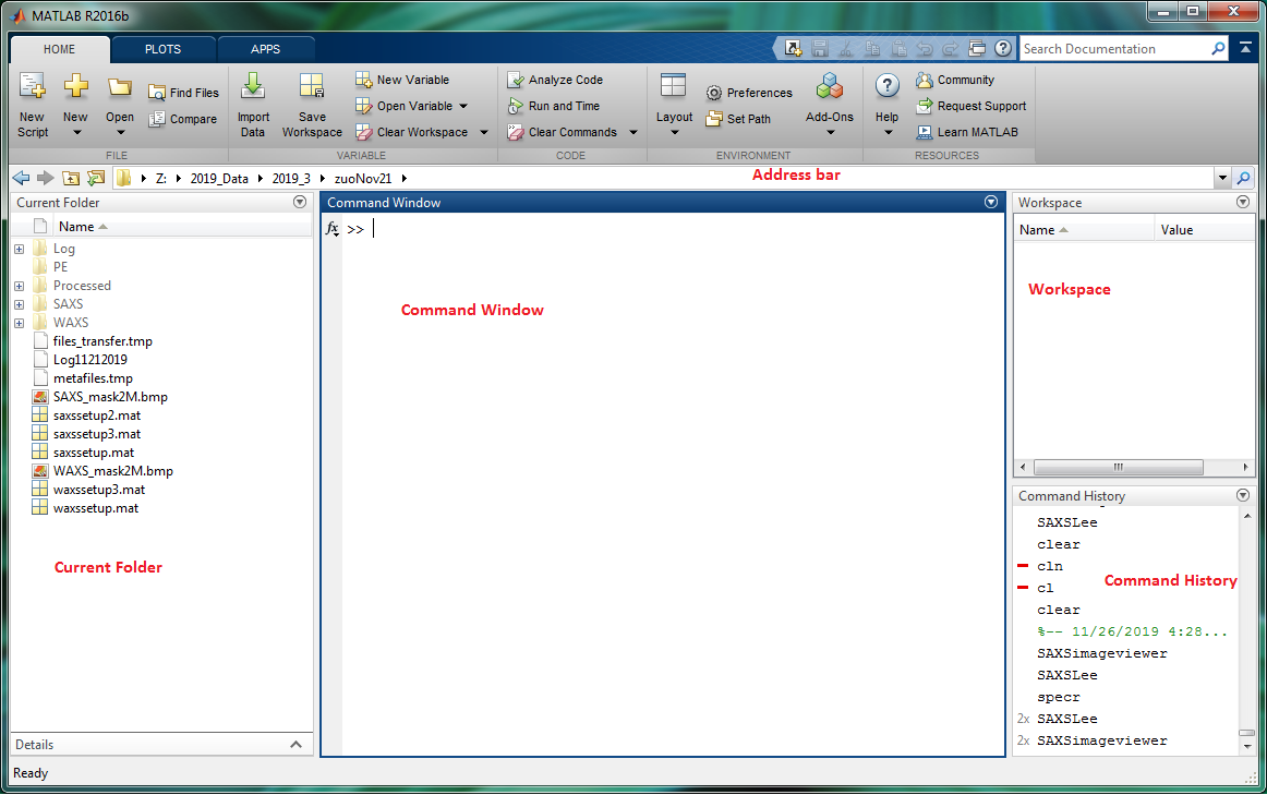
Double-click the Matlab icon at the Desktop, you will get the Matlab Window like Figure 1. From the Address bar, navigate to your data folder. In your Data Folder, you will have several folders, i.e., "SAXS" folder --for SAXS data; "WAXS" --for WAXS data; "PE" --for perkinElmer detector data; "Log" --log files for your image data measurements.
Figure 1. Matlab program window. "Current Folder" displays folders and files under your folder. You can run matlab functions and commands in "Command Window" . "Workspace" shows the matlab parameters in memory. "Command History" displays commands/operations run recently in "Command Window"; you can double-click the command to run it from the history list.
2. Start 2D Image Visualization Program
Execute (type and hit enter) “SAXSimageviewer” in the matlab "Command Window" and you will get the matlab graphic window "SAXSIMAGEVIEWER" for 2D image visualization. The command could also be run in the “Command History” sub-window.
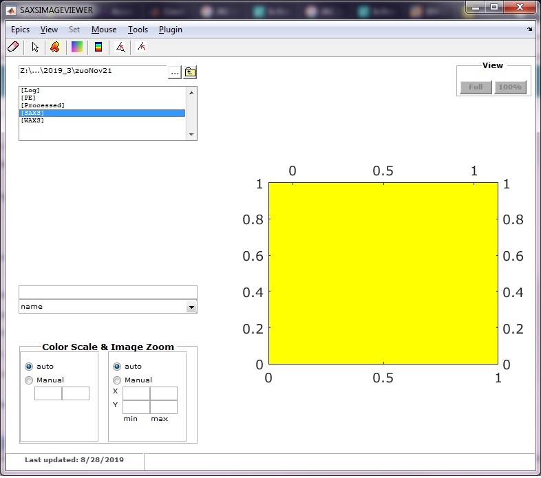
Figure 2A SAXSimageViewer
Choose an image data folder - for instance, "SAXS". Under menu "Plugin", click "Experiment Setup" - a matlab GUI program "GISAXSshop" will pop up. Images can be listed by "name", "date", "bytes", or "datenum". Listing by "date" is recommended, which puts the most recent one at the top. Click any image file to display.
To update the image data list, hit "enter" in the circled box. Also can use patterns (such as "*", "Swat*", "*_00021_*") this box to narrow down search.
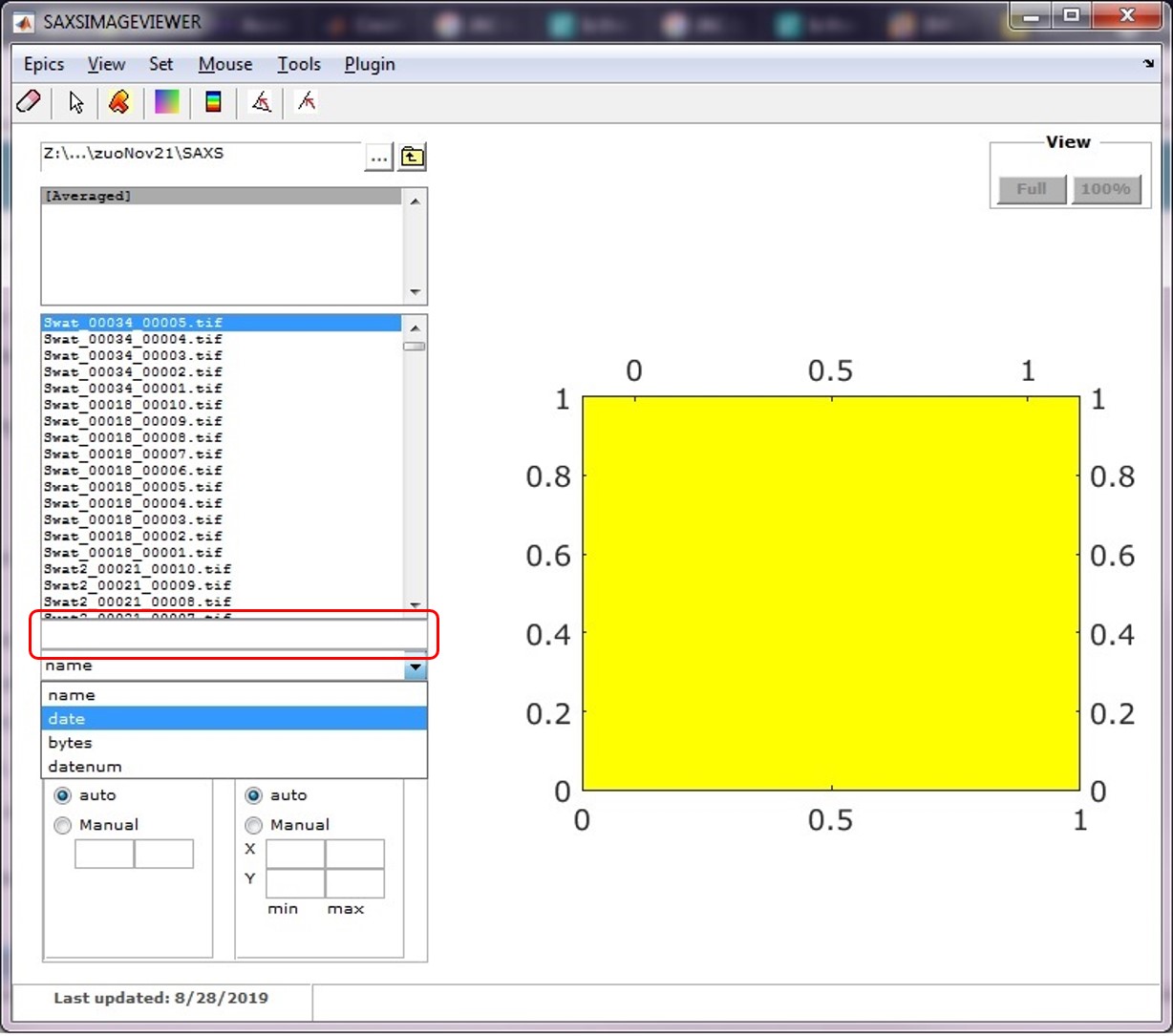
Figure 2B
Click the square color icon to switch image color scales between log and linear scales. This can also be done through "View" menu. There are choices of "auto" and "Manual" for Color Scale at left bottom; "Manual" with range of [0, 5] is recommended.
There are two choices for Image Zoom - "auto" and "Manual". "auto" will display the whole image; "Manual" will show specified area. With the cursor on the image display, use the left mouse button to drag the image (pan motion), and use the right mouse button to zoom in/out.
Under menu "Epics", you can specify image data from which detector ("Pilatus2M", "PerkinElmer", or "Mar 300") will be automatically updated in the display window.
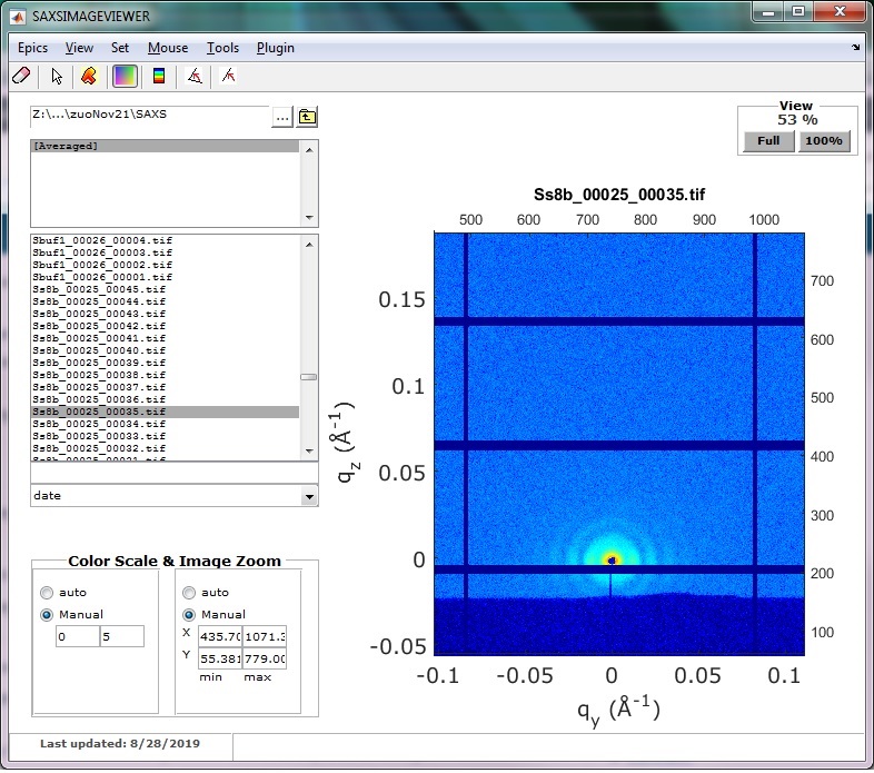
Figure 2C
3. Start GISAXSshop Program
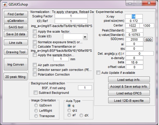
Figure 3. GISAXSshop/gisaxsleenew program screen
This program is needed for SAXSIMAGEVIEWER to correctly display 2D images.
To start it, click "Experiment Setup" from "Plugin" menu in SAXSIMAGEVIEWER, or execute “gisaxsleenew” from "Command Window" or "Command History".
Input parameters in "Experimental setup" section, or load them using "Load setup info" button if pre-saved info exists. After experimental setup information is available, the q_x, and q_y values will be computed and displayed in the 2D image window (Figure 2C). Then, the q value at every pixel will become available and ready to check using mouse cursor.
4. Detector Q-& Absolute Intensity Calibration, and 2D Data Conversion Program
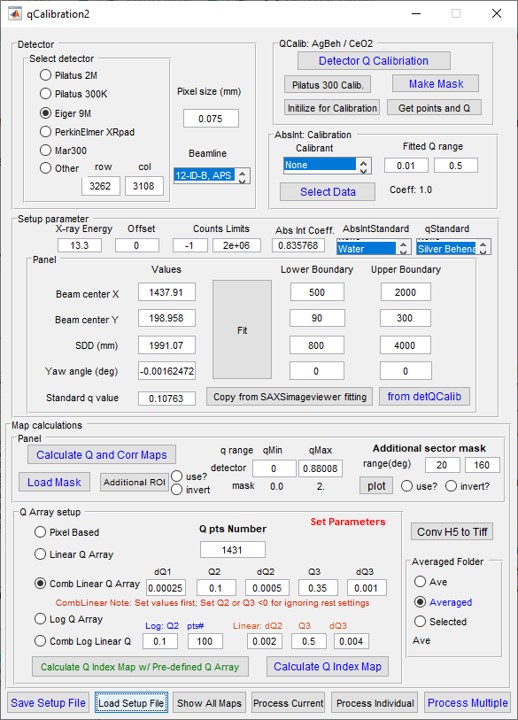
Figure 4. qCalibration2 program GUI
To load the program, type "qCalibration2" and hit " Enter " key in the main matlab "Command Window", and the left GUI program screen will pop up.
qCalibration2 can: (1) calibrate Q-values for area detectors; (2) calibrate absolute intensity; (3) prepare setup file for 2D image data conversion; (4) convert 2D image data to 1D scattering data.
To convert 2D image data: (1) "Load Setup File" to load pre-made setup parameter file; (2) choose desired destination folder in "Averaged Folder"; (3) press "Process Multiple" botton to select image files and the program will automatically process them.
Note: (a) If you want to change the number of q points to have more (finer q resolution) or less(for better S/N) data points, make the proper selection in the "Q Array setup", then "Calculate Q index Map", then run "Process Multiple".
(b) Applying additional ad hoc region of interest(ROI) or mask for the data conversion is possible in this program. There are two choices which can be applied independently: "Additional ROI" for arbitrary polygon ROI/mask, and Sector ROI/mask. After preparing and choosing the proper ROI/masks, run "Process Multiple". The selected ROI/masks, will be applied to the existing mask in the setup file.
5. Start 1D Data Visualization Program
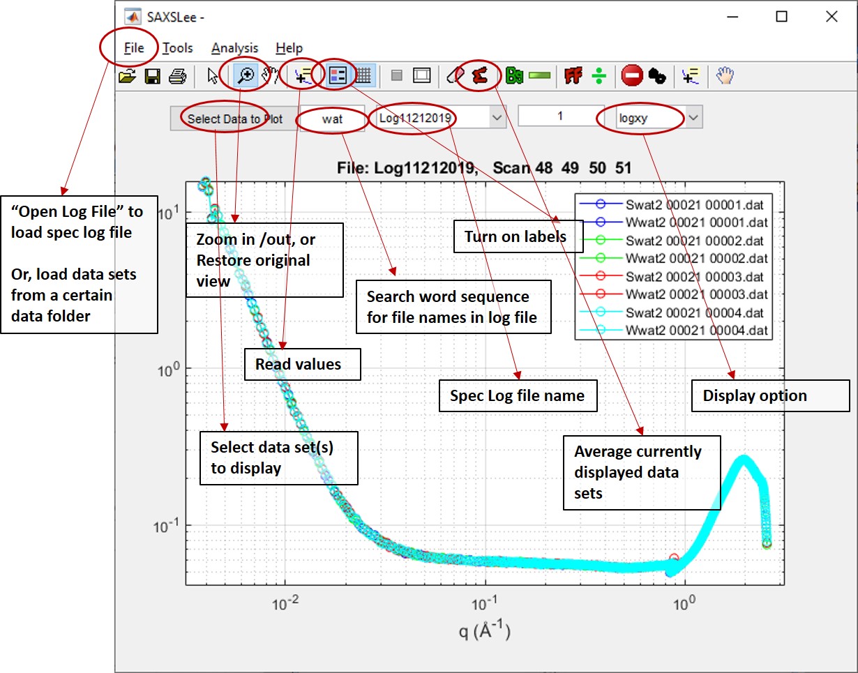
Figure 5. SAXSLee program GUI
To view the converted 1D profiles, type “SAXSLee” and hit "Enter" key in the main matlab "Command Window", and you will get the following GUI program screen.
Under the "File" menu, click "Open Log File..." to load the spec log file. The spec log file is starting with "Log", followed by the first experimental date, for example, "Log11212019".
Spec log file contains records of sample measurements and motor scans. Do NOT modify the spec log file! It may mess up data collection!
When the program loads the spec log file, it reads data file names from the spec log file. At 12-ID, 2D images will be automatically converted to 1D curvers. Both will be saved to your data folder. Now, you can start to look your 1-D data through "Select Data to Plot". The program screen also provides other functions, such as zooming, reading data point value, displaying options (linear, log), averaging, and subtraction.
6. View Motor Scan Profile
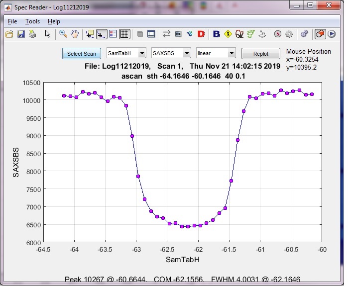
Figure 6. specr program GUI
To view the motor scan, type "specr" in the main matlab "Command Window", and you will get the following GUI program.
Under the "File" menu, click "Open Log File" to load the spec log file, then you can start to look your data through "Select Scan".
Additional instruction videos available:
- Intro to SAXSimageviewer
- q Calibration with SAXSimageviewer and gisaxsleenew
- Making a mask image
- Linecut and/or Azimuthal Averaging
- Absolute Intensity Calibration with SAXSimageviewer and gisaxsleenew
- Intro to SAXSLee I (Background Subtraction, Data Merging, etc)
- Intro to SAXSLee II (Simple Data Analysis)
Install Matlab package
The Matlab package is available to 12-ID users upon request for outside beamline use.
(1) Save the 12-ID-B matlab package in a desired folder, and unzip the package.
(2) Add the matlab package into the matlab path, through "Set Path" and "Add with Subfolder", see below:
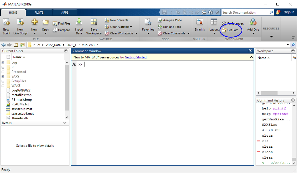
Click "Set Path" in Matlab to find the folder containing the matlab package. This leads to the below interface:
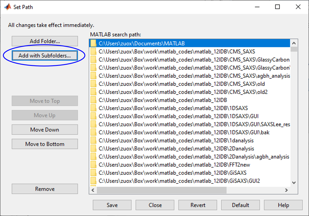
"Add with Subfolder" to add the matlab package into the searching path. Then "Save" and "Close".
Set up HDF5 Plugin
Data collected at Sector 12-ID are now in hdf5 format with compression on 2-D image data. In order to read the 2-D image data using the matlab package, one needs: (1) a matlab with version of 2020 or later, (2) installation of HDF5 plugin from the HDF Group . The latest package has already included the hdf5 plugins. To set them up, start the Matlab software first, then run "set_hdf5_plugins" in the Command Window, as shown in the figure below. If the setup conpletes successfully, close Matlab and restart it. The matlab package will then be ready to use.
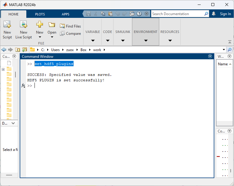
Command to set up HDF5 plugins and Messages
Alternative way to install HDF5 plugin
HDF5 plugins are now distributed as part of the HDF5 library or HDFView, which can be obtained from The HDF5 Group Website. Once installed, find the hdf5 plugin folder, and configure as the follow.
For Windows users, the HDF5 plugin environment variables are needed to set through: "Control Panel" --> "System and Security" --> "System" --> "Advanced system settings" --> "Environment Variables"
Set Variables "HDF5_DIR", "HDF5_PLUGIN_PATH", and "LD_LIBRARY_PATH" using "NEW" or "Edit", like below:
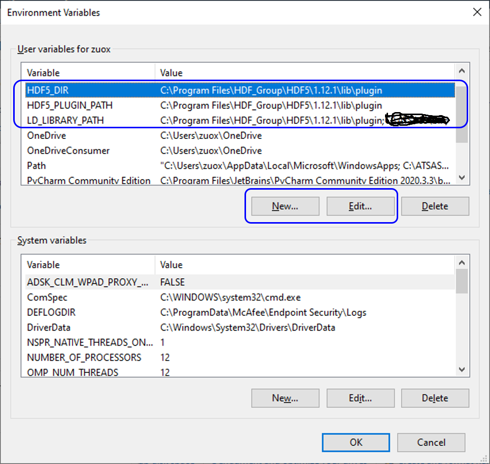
Then "OK" to save. Try if you can open image data file from "SAXSIMAGEVIEWER". If not, add "HDF5_DIR", "HDF5_PLUGIN_PATH", and "LD_LIBRARY_PATH" in "System variables", which may need admistrator privilege.
Installation Instruction for other OS can be found here: Installation instruction